What really is vectorization and how does it work?

In machine learning, or in computer science/engineering literature we sometimes read about improving runtime performance with vectorization. We hear a lot about it with the way typicall machine learning libraries work such as numpy or pandas.

But what really is vectorization and how does it work in practice?

SIMD

One of the ways to perform vectorization is when your program is compiled to vectorized CPU instructions. This type of parallel processing is called Single Instruction Multiple Data (SIMD) under Flynn’s Taxonomy.

But what are vectorized CPU instructions? Modern CPU’s support multiple instruction sets extensions which implement SIMD.

Examples of these sets are MMX, SSE, AVX, etc… and are available on modern Intel and AMD CPU’s. These instruction sets were developed and improved along the years of microprocessure architecture development.

For an historical reference, AVX was extended into AVX2 for the first time in 2013 when Intel launched the Haswell microprocessor architecture.

Comparison between non-vectorization and vectorization behaviour

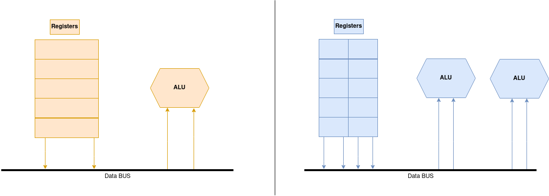
A normal machine cycle will include the Fetching Stage where the CPU will fetch the instruction and data from the registers, it will then decode the instructions in the Decoder Stage and emit the relevant signals to the ALU in the Execution Stage. An ALU(Arithmetical Logic Unit) is a digital circuit which is responsible for arithmetical operations on operands.

In the figure below the Decoder Stage is omitted. Normal registers have a fixed bit length dimension where data is stored, and if an operation takes two operands an ALU will perform an operation on these 2 operands during the Execution Stage.

In a vectorized architecture, vectors are stored in Vector Registers which behave similarly to Scalar Registers and are divided into a fixed number of chunks supporting more than one variable.

E.g if we had a scalar register of 128 bits, a similar vector register could store 4 elements of 32 bits.

Loading data from a register will load multiple elements at a time, in one single machine cycle. Modern CPU’s support multiple ALU’s and so we can perform multiple independent operations in parallel.

vectorization

Hinting the compiler

Now the question is how can we hint the compiler to compile our code with a vectorized instruction set. We will explore 2 options:

Vector Intrisics
Auto Vectorization

I made a proof of concept Github Repository which you can explore.

Lets take as an example the task of multiplying two square matrices. Each matrix is a floating pointer flat array and the matrix is stored in row-major.

void matrixMultiplication(float* first, float* second, float* result){
    for(int i = 0; i < array_size; ++i){
        for(int j = 0; j < array_size; ++j){
            result[i*array_size + j] = 0;
            for(int k = 0; k < array_size; ++k){
                result[i*array_size + j] += first[i*array_size + k] * second[k*array_size + j];
            } 
        }
    }
}

The code above implements the standard matrix multiplication algorithm (without any improvements) whose time complexity is O(n³).

Vector Instrisics

Vector intrisics feel like regular functions you call in normal C++ source code, but they are compiler intrisic functions meaning that they are implented directly in the compilers. They are useful since they help hint the compiler to use vectorized instructions, since the compiler has a intimate knowledge of the function and can integrate it and optimize it for better usage.

The vector intrisics you’ll see below either finish with ss or ps. That is because ss stands for scalar instructions and ps stands for packed instructions. Packed operations operate on a vector in parallel with a single instruction while scalar instructions operate only one element.

Some of the operations below need to be performed on 32 byte aligned memory addresses (or 16 in case of 4 packed operations) which means that the memory address needs to be divisable by 32.

void vectorizedMatrixMultiplication4(float* first, float* second, float* result){
    for(int i = 0; i < array_size; i++){
        for(int j = 0; j < array_size; j+=4){
            __m128 row = _mm_setzero_ps();
            for(int k = 0; k < array_size; k++ ){
                // fetches the element referenced by the pointer and broadcasts it into a vectorized scaled single precision.
                // Since its row X column, the each row element will have to be multiplied by each member of the column.
                __m128 first_packed = _mm_broadcast_ss(first + i * array_size + k);
                // row of the second matrix.
                __m128 second_packed = _mm_load_ps(second + k*array_size + j);
                __m128 multiplied_packed = _mm_mul_ps(first_packed, second_packed);
                row = _mm_add_ps(row, multiplied_packed);
            } 
            _mm_store_ps(result + i*array_size + j, row);
        }
    }

In the code above we used 6 intrisics:

_mm_set_zero_ps: Create a vector of 4 zeros.
_mm_broadcast_ss: Broadcast an element pointed by first + i * array_size l + 4 times to the array.
_mm_load_ps: Load 4 consequentive floating type numbers from a 16 byte aligned memory address.
_mm_mul_ps: Vectorized multiplication
_mm_add_ps: Vectorized addition
_mm_store_ps: Store the resulting calculation of 4 numbers in a memory address.

All these operations return or interact with __m128 types which is a packed vector type holding 4 32-bit floating point values, which the compiler will store on vector registers.

void vectorizedMatrixMultiplication8(float* first, float* second, float* result){
    for(int i = 0; i < array_size; i++){
        for(int j = 0; j < array_size; j+=8){
            __m256 row = _mm256_setzero_ps();
            for(int k = 0; k < array_size; k++ ){
                // fetches the element referenced by the pointer and broadcasts it into a vectorized scaled single precision.
                // Since its row X column, the each row element will have to be multiplied by each member of the column.
                __m256 first_packed = _mm256_broadcast_ss(first + i * array_size + k);
                // row of the second matrix.
                __m256 second_packed = _mm256_load_ps(second + k*array_size + j);
                __m256 multiplied_packed = _mm256_mul_ps(first_packed, second_packed);
                row = _mm256_add_ps(row, multiplied_packed);
            } 
            _mm256_store_ps(result + i*array_size + j, row);
        }
    }
}

Similarly, in the code above we used 6 intrisics:

_mm256_setzero_ps: Create a vector of 8 zeros.
_mm256_broadcast_ss: Broadcast an element pointed by first + i * array_size l + 8 times to the array.
_mm256_load_ps: Load 8 consequentive floating type numbers from a 32 byte aligned memory address.
_mm256_mul_ps: Vectorized multiplication
_mm256_add_ps: Vectorized addition
_mm256_store_ps: Store the resulting calculation of 4 numbers in a memory address.

All these operations return or interact with __m256 types which is a packed vector type holding 8 32-bit floating point values, which the compiler will store on vector registers.

For more vector intrisics check Intel intrisic guide.

Auto Vectorization

Assembly code comparison

We can debug the assembly file result of the compilation process with g++ -S ... before assembling and linking it.

For a simple matrix multiplication let’s take a look at part of the assembly code generated by the compiler.

_Z20matrixMultiplicationPfS_S_:
(...)
.L8:
	movl	-12(%rbp), %eax
	imull	$1600, %eax, %edx
	movl	-8(%rbp), %eax
	addl	%edx, %eax
	cltq
	leaq	0(,%rax,4), %rdx
	movq	-40(%rbp), %rax
	addq	%rdx, %rax
	movss	(%rax), %xmm1
	movl	-12(%rbp), %eax
	imull	$1600, %eax, %edx
	movl	-4(%rbp), %eax
	addl	%edx, %eax
	cltq
	leaq	0(,%rax,4), %rdx
	movq	-24(%rbp), %rax
	addq	%rdx, %rax
	movss	(%rax), %xmm2
	movl	-4(%rbp), %eax
	imull	$1600, %eax, %edx
	movl	-8(%rbp), %eax
	addl	%edx, %eax
	cltq
	leaq	0(,%rax,4), %rdx
	movq	-32(%rbp), %rax
	addq	%rdx, %rax
	movss	(%rax), %xmm0
	mulss	%xmm2, %xmm0
	movl	-12(%rbp), %eax
	imull	$1600, %eax, %edx
	movl	-8(%rbp), %eax
	addl	%edx, %eax
	cltq
	leaq	0(,%rax,4), %rdx
	movq	-40(%rbp), %rax
	addq	%rdx, %rax
	addss	%xmm1, %xmm0
	movss	%xmm0, (%rax)
	addl	$1, -4(%rbp)
(...)

_Z31vectorizedMatrixMultiplication4PfS_S_:
(...)
.L19:
	movl	-180(%rbp), %eax
	imull	$1600, %eax, %eax
	movslq	%eax, %rdx
	movl	-172(%rbp), %eax
	cltq
	addq	%rdx, %rax
	leaq	0(,%rax,4), %rdx
	movq	-200(%rbp), %rax
	addq	%rdx, %rax
	movq	%rax, -160(%rbp)
	movq	-160(%rbp), %rax
	vbroadcastss	(%rax), %xmm0
	nop
	vmovaps	%xmm0, -128(%rbp)
	movl	-172(%rbp), %eax
	imull	$1600, %eax, %eax
	movslq	%eax, %rdx
	movl	-176(%rbp), %eax
	cltq
	addq	%rdx, %rax
	leaq	0(,%rax,4), %rdx
	movq	-208(%rbp), %rax
	addq	%rdx, %rax
	movq	%rax, -168(%rbp)
	movq	-168(%rbp), %rax
	vmovaps	(%rax), %xmm0
	vmovaps	%xmm0, -112(%rbp)
	vmovaps	-128(%rbp), %xmm0
	vmovaps	%xmm0, -48(%rbp)
	vmovaps	-112(%rbp), %xmm0
	vmovaps	%xmm0, -32(%rbp)
	vmovaps	-48(%rbp), %xmm0
	vmulps	-32(%rbp), %xmm0, %xmm0
	vmovaps	%xmm0, -96(%rbp)
	vmovaps	-144(%rbp), %xmm0
	vmovaps	%xmm0, -80(%rbp)
	vmovaps	-96(%rbp), %xmm0
	vmovaps	%xmm0, -64(%rbp)
	vmovaps	-80(%rbp), %xmm0
	vaddps	-64(%rbp), %xmm0, %xmm0
	vmovaps	%xmm0, -144(%rbp)
	addl	$1, -172(%rbp)
(...)

These figures above show part of the instruction set used in the assembly result of our c++ code. You can notice the difference in the used instruction set from the traditional matrix factorization (_Z20matrixMultiplicationPfS_S_) to the vectorized one (_Z31vectorizedMatrixMultiplication4PfS_S_).

Two very quick examples are the usage of imull and addl in contrast with vmulps and vaddps respectively.

Auto-Vectorization

Auto-vectorization essentially means that we let the compiler optimize our calculation loops by itself, without hinting, which will work for traditional cases.

Take a loot at the following command: g++ -ftree-vectorize -mavx ...

We’re only aiming for vectorization, so we will omit level 3 optimization (-O3) and that’s what the ftree-vectorize compiler flag stands for.

We also need to target a valid SIMD instruction set extension so that it can be used by the compiler. That’s what the -mavx flag does.

Execution time comparison

The results below were done for a squared matrix of 1600 by 1600.

Function	Average Time
Simple Matrix Factorization	14933 ms
Auto-Vectorization	11962 ms
Vectorized Matrix Multiplication (4)	9817 ms
Vectorized Matrix Multiplication (8)	6143 ms

References

André Fernandes

What really is vectorization and how does it work?