Gradient boosting trees

In this post we will analyse how gradient boosting regression trees work under the hood, and go over some code samples taken from my Github repo.

Regression trees

Regression trees are an application of decision trees used in machine learning for applying regression tasks on a series of data points. They work similarly to standard classification trees but instead of using categorical data, they use continuous labels. They can also be interpreted as a list of hierarhical if-else statements applied on data features.
They are buil in a binary fashion where a node can have at-most 2 child nodes (or leaves).
Tree balance depends on implementation stopping criteria for building trees. Few ideas below:
- If stopping criteria defines a maximum tree level to be reached, trees will grow left and right side nodes until that maximum level is reached.
- You can also establish a maximum number of nodes where if a maximum number of nodes is reached, trees will stop growing.
- It is also possible, to grow trees by number of leaves and greedily explore nodes which decrease error the most.
- I.e The public package lightgbm grows trees leaf-wise instead of level-wise.

The heuristic is the following:

Create root node.
Check for stopping criteria -if not reached continue, else exit.
Find best split feature.
Make recursive call, depending on implementation.

Notice the implementation at the abstract node builder class and the tree-level node builder subclass.

def build(self, points: np.array, labels: np.array) -> Node:
        if self.should_stop(points=points):
            node_id = self._node_count
            self._node_count += 1
            return Node(node_id=node_id, threshold=labels.mean())

        return self.recursive_call(points=points, labels=labels)

 def recursive_call(self, points: np.ndarray, labels: np.ndarray) -> Node:
        """
        The function recursive call on building the tree level-wise. Overriding the
        parent class and finding the best feature split greadily.

        Arguments:
            points: numpy array The current level data points across all features.
            labels: numpy array The labels for the respective points.
        """
        feature_split, lhs, rhs = find_best_split(points=points, labels=labels)
        feature_idx, threshold_value, _ = feature_split
        lhs_points, lhs_labels = lhs
        rhs_points, rhs_labels = rhs

        self._current_level += 1
        left = self.build(points=lhs_points, labels=lhs_labels)
        right = self.build(points=rhs_points, labels=rhs_labels)

        return Node(node_id=self._node_count, split=(feature_idx, left, right), threshold=threshold_value)

We start by checking if we should_stop and return a new Node object when we meet the criteria. If we do not, we find the best split feature (more on that later) and check for the left-hand side and right-hand side points to continue splitting. Then we make 2 recursive calls, one for the left-hand side child and right-hand side child increasing the level count self._current_level += 1. The process is repeated until the stopping criteria is met.

In order to find the best split we need to check 2 things:

How do we measure what is “best” ?
For each feature what is the best threshold for splitting.
What is the best feature for splitting.

In the linked implementation we order the continuous points in order to find the best pair of points (mean) which minimizes the total loss computed by summing:

Left-hand-side loss - Mean of the labels of the left-hand-side of the assessed pair threshold
Right-hand-side loss - Mean of the labels of the right-hand-side of the assessed pair threshold

    # split area
    lhs = labels[:candidate_treshold_idx]
    rhs = labels[candidate_treshold_idx:]

    # split predictions
    pred_lhs = lhs.mean()
    pred_rhs = rhs.mean()

    # mse split loss
    lhs_loss = (lhs - pred_lhs).sum()
    rhs_loss = (rhs - pred_rhs).sum()
    total_candidate_loss = np.abs(lhs_loss + rhs_loss)

We then compute this for all features and find the best split greedily. This is known as the CART algorithm.

for feature_idx in range(n_features):
        feature = points[:, feature_idx]
        feature_sorted_idx = sorted_idx[:, feature_idx]
        # use sorted feature to find the best split
        candidate_idx, candidate_value, candidate_ft_loss = find_best_split_feature(
            feature=feature[feature_sorted_idx], labels=labels[feature_sorted_idx]
        )

        if min_feature_loss is None or candidate_ft_loss < min_feature_loss:
            min_feature_loss = candidate_ft_loss
            best_loss_feature = feature_idx
            threshold_idx = candidate_idx
            threshold_value = candidate_value

We then return the best split:

# return feature spit, left and right split
feature_split = FeatureSplit(best_loss_feature, threshold_value, min_feature_loss)
lhs = HandSide(lhs_points, lhs_labels)
rhs = HandSide(rhs_points, rhs_labels)

As an example:

import seaborn as sns
import numpy as np
import pandas as pd
import matplotlib.pyplot as plt
import plotly.express as px


from gradient_boosting_trees.model import GBRegressionTrees, GBParams
from gradient_boosting_trees.regression.tree import RegressionTree
from gradient_boosting_trees.regression.cart.builder import TreeLevelNodeBuilder

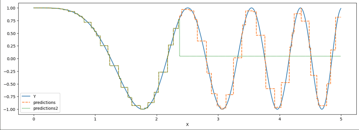
X = np.arange(5, step=0.001)
Y = np.cos(X**2)
X = X.reshape(len(X), 1)
data = pd.DataFrame(list(zip(X.ravel(), Y)), columns=["X", "Y"])

builder = TreeLevelNodeBuilder(min_moints=150, max_level=100)
tree = RegressionTree(node_builder=builder)

builder_2 = TreeLevelNodeBuilder(min_moints=150, max_level=50)
tree_2 = RegressionTree(node_builder=builder_2)

tree.fit(points=X, labels=Y)
tree_2.fit(points=X, labels=Y)

predictions = tree.predict(X)
predictions2 = tree_2.predict(X)

data["predictions"] = predictions
data["predictions2"] = predictions2

tree

Gradient Boosting

Gradient boosting is an ensembe technique which involves a list of “weak-learners” whose composed training forms a “stronger” model. In training, at each step a new weak model trained on the gradient of the error of the current strong model and then added to the least of weak learners.

Mi+1 = Strong model at ith iteration + 1
Mi = Strong model at ith iteration
mi = Weak model at ith iteration

Mi+1 = Mi - mi

In our implementation in the GBRegressionTree class we zero-initialize the strong model strong_predictions and create an empty list with the weak models which will be RegressionTree objects.

We then compute the gradient of the squared error with regards to the current strong predictions and labels and fit the current regression tree of the current iteration to that gradient. After that, we get the predicitons of the tree and iteratively modify the current strong predictions with the weak predictions we get from the weak model multiplied by a shrinkage parameter.

strong_predictions = np.zeros_like(labels)
self._weak_models = []

for _ in tqdm(range(n_iterations)):
    error = squared_error(raw_predictions=self.predict(points=points), labels=labels)
    self.learning_error.append(error)

    gradient, hessian = squared_error_gradient_hessian(raw_predictions=strong_predictions, labels=labels)

    self._builder.reset()
    tree = RegressionTree(node_builder=self._builder)
    tree.fit(points=points, labels=gradient)
    self._weak_models.append(tree)

    weak_predictions = tree.predict(points=points)
    strong_predictions -= self._params.shrinkage * weak_predictions / hessian

Notice as well we also compute an hessian, being the second-order derivative, of the error (constant array in our-case), which is referred as the Newton-trick or Newton-raphson method application in gradient boosting (In this case, second-order approximation is really not needed since we can get by with just modifying the shrinkage parameter).

params = GBParams(shrinkage=0.001)
builder = TreeLevelNodeBuilder(min_moints=150, max_level=150)
gradient_boosting  = GBRegressionTrees(params=params, node_builder=builder)

X = np.arange(20, step=0.01)
Y = np.cos(X)
X = X.reshape(len(X), 1)

gradient_boosting.fit(points=X, labels=Y, n_iterations=200)
gb_predictions = gradient_boosting.predict(points=X)

builder = TreeLevelNodeBuilder(min_moints=150, max_level=100)
tree = RegressionTree(node_builder=builder)
tree.fit(points=X, labels=Y)

tree_preds = tree.predict(X)

plt.figure(figsize=(15, 5))

data = pd.DataFrame(index=X.ravel(), data=list(zip(Y, gb_predictions, tree_preds)), columns=["True Y", "Gradient Boosting", "Regression Tree"])
sns.lineplot(data=data)

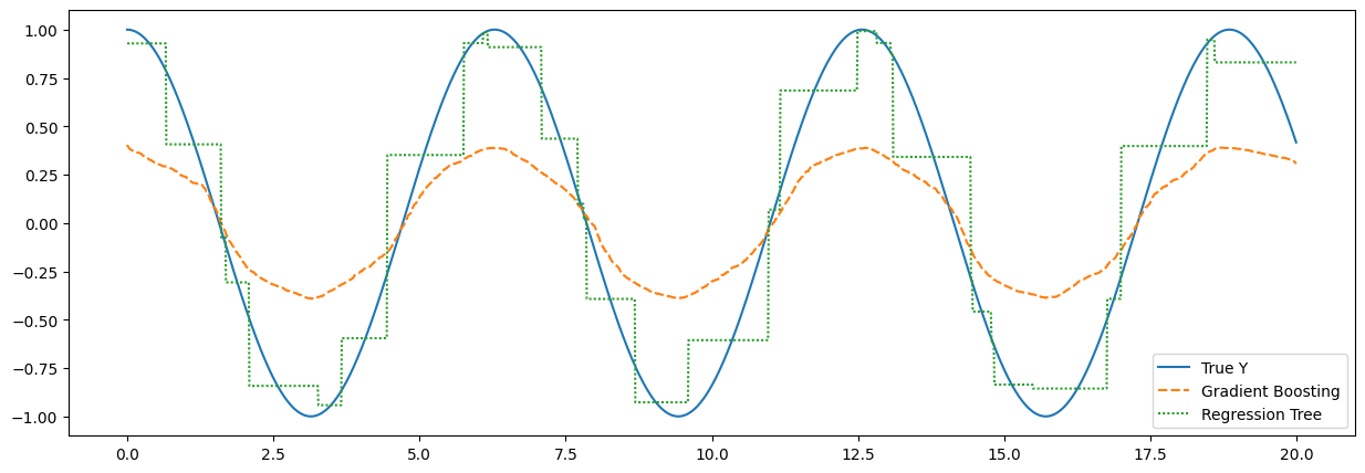
Notice how the predictions of a simple regression tree are done by threshold evaluation of the provided X values which could be simply defined as if-else statements and the prediction line resembles a step-function. In contrast, the gradient boosting predictions offer a smoother line, made of the contributions of each one of the weaker regression trees.

André Fernandes

Gradient boosting trees